Models

Jump to: Life-cycle assessment models | Process-based models | Proxy indicators

Empirical models

Regression analysis can be used to extrapolate existing research and data to develop empirical models that describe explicit GHG emissions and carbon sequestration factors as a function of agriculture activities. Empirical models are relatively easy and transparent to use. However, they are not appropriated to capture the effects of spatial and temporal variability on GHG dynamics at finer scales. They are also less flexible to handle combinations of variable management (Olander & Haugen-Kozyra, 2011).

Shcherbak et al. (2014), for example, performed a meta-analysis using 78 published studies (233 site-years) with at least three N-input levels to estimate N₂O emission factors (EFs). The statistical analysis revealed that the N₂O response to N inputs grew significantly faster than linear for synthetic fertilizers and most crop types. Therefore, this analysis helped improve the EF provided by the IPCC Tier 1 method that assumes a linear relationship between N input and N₂O emissions (Fig. 1).

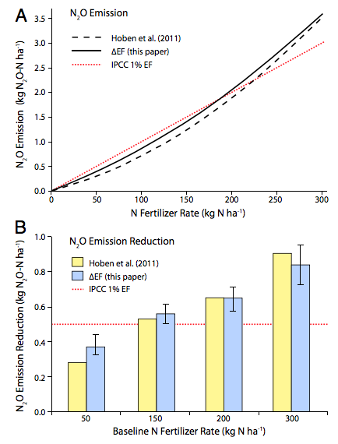
Figure 1. (A) Comparison of N2O emission models for N fertilizer reduction scenarios: N2O emissions estimated by the IPCC Tier 1 (1% linear emission) model, the Hoben et al. (2001) model (0.001 N[4.36 + 0.025 N]), and the ΔEF model for average upland grain crop emissions from this meta-analysis (0.001 N[6.49 + 0.0187 N]). (B) Relative N2O emission reductions for the three models when N fertilizer rates are reduced by 50 kg ha−1 from four baseline N fertilization scenarios: 300, 200, 150, and 50 kg ha−1. Vertical lines denote SEs for emission estimates based on the ΔEF model (Shcherbak et al., 2014).

Life-cycle assessments (LCA)

A life-cycle assessment (LCA) is a quantitative method for determining GHG emissions or removals and other environmental impacts and resource demands across a product’s entire supply chain. An LCA framework can determine areas of most significant impact and compare reduction strategies for agricultural production systems.

Initially developed for industrial operations, the LCA methodology has been expanded to a broader range of fields, including agriculture. An LCA may be conducted in agriculture, for example, for food products or supply chain equipment. The assessment boundaries may range from “cradle” to “grave” or only for parts of this range or product’s life cycle.

• ISO 14040-14044: this methodology specifies requirements and provides extensive and detailed guidelines for LCA.
• USDA Ag Data Commons – Life Cycle Assessment: this is a catalog and archive of data, tools, and resources that support LCA for agriculture and related areas of research. This is complementary to the USDA-LCA Commons Life Cycle Inventory (LCI) database and provides access to a wider range of LCA data and tools.
• Gleam: The Global Livestock Environmental Assessment Model (GLEAM) is a global information system (GIS) framework for simulating the biophysical processes and activities in livestock supply chains using an LCA approach.

Process-based models

A process-based model is the mathematical representation of biogeochemical processes characterizing the functions of an agroecosystem, including greenhouse gas emissions and carbon sequestration.  The models are created based on substantial long-term research and can be used in two distinct ways: at local/farm and regional levels (Olander & Haugen-Kozyra, 2011).

Process-based models may provide the most cost-effective manner of quantifying GHG emissions from agricultural activities and evaluate mitigation options at a large scale. However, process-based models require more detailed data and technical capacity for model parameterization and calibration. Hence, process-based models are usually complex and, therefore, its process is not well transparent.

Major process models for crop, grassland, and livestock systems include:

• DNDC: the DeNitrification-DeComposition model (DNDC) is a family of models for predicting plant growth, soil C sequestration, GHG emissions, and nutrient fluxes for cropland, pasture, forest, wetland, and livestock operation systems.
• DayCent/CENTURY: the DAYCENT model simulates the C and N fluxes among the atmosphere, vegetation, and soil interactions. This model is the daily time-step version of the CENTURY biogeochemical model.
• Roth-C: a model for the turnover of organic carbon in topsoil, allowing for the effects of soil (i.e. type, temperature, moisture), plant and agriculture management characteristics on the turnover process.
• EPIC-APEX: The Environmental Policy Integrated Climate (EPIC) is a cropping systems model that estimates soil productivity as affected by erosion, whereas the Agricultural Policy/Environmental eXtender (APEX) model was designed to extend the capabilities of the EPIC model to simulate impacts on land management in small-medium watersheds and a variety of farms.
• NASA-CASA: the NASA-CASA model simulates net primary production and soil heterotrophic respiration at regional to global scales.
• APSIM: the agricultural production systems simulator (APSIM) estimates biophysical processes of a range of agricultural systems.
• RUMINANT: is an animal-level model that simulates the effects of nutrition (feed quality and availability) on the growth and production of cattle, sheep, and goats.

Proxy indicators

Proxy indicators for estimating GHG emissions rely on statistical relationships among agricultural management factors at individual, farm, or landscape levels and associated GHG emissions and removals. They allow the use of a simple indicator of GHG emissions and thereby avoid more costly measurements. Indicators are ideally those that farmers already monitor, such as yields.

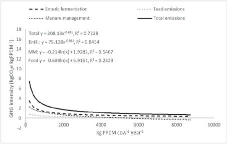
For example, milk yield can be used as an indicator of the emissions in livestock systems. Plotting kg of fat and protein corrected milk (FPCM) per cow against GHG intensity (kgCO2e/kg FPCM) on smallholder farms in central Kenya, Wilkes et al. (2020) shows that differences in GHG intensity among individual cows are explained largely by milk yield performance (R2 = 0.72). Milk yield is related to enteric fermentation emissions (R2 = 0.84), manure management emissions (R2 = 0.54) and the emissions embodied in animal feed (R2 = 0.23; Fig. 2).

While these indicators reduce the costs of monitoring GHG emissions, they can have significant errors. Errors are most likely because of inter-household differences in the adoption of agricultural practices (i.e., improved genetics, nutrition and animal health), which are generally greater on smallholder farms in developing countries than developed contexts (Mayberry et al., 2017). For example, Wilkes et al. (2020) indicated a ±16% error in the carbon footprint of dairy smallholder farms in Kenya due to input variability. This error was similar to the error found in a study with dairy smallholder farms in India (Garg et al., 2016). However, it was larger than reported in North America, Oceania and Euronpean dairy farms (O’Brien et al., 2012; Jayasundara et al., 2019; Gollnow et al., 2014) – which ranged between ±2.5% and ±4.0%.

Therefore, the proxy indicator’s accuracy should be considered, and potential trade-offs should be taken into account, especially when applied to climate financial contexts, such as carbon markets (see Gold Standard – Carbon Market Methodology).