Why low-emissions development (LED) in agriculture?

Low-emission development (LED) in agriculture refers to the aim of improving economic, social, or environmental conditions in the production of crops or livestock while also contributing to climate change mitigation. Mitigation in this context is a co-benefit of agricultural production. Some refer to low-emission development as a decoupling of economic growth from GHG emissions growth or as climate-compatible development (GIZ 2013).

International development programs for agriculture often produce mitigation co-benefits, even without having a mitigation objective (Grewer et al. 2019, Costa Jr. et al. 2020, Richards et al. 2019)(Figure 14). Analysis of the mitigation impacts of agricultural investments of the US Agency for International Development (USAID), the UK Department for International Development (DfID) (now Foreign Common Wealth and Development Office), and the International Fund for Agricultural Development (IFAD) showed consistent net mitigation impacts across each of their portfolios.

A sample of DfID’s investments showed that even at the level of a single program, food value chains increased average crop productivity by 1.0 ton per hectare per year, but reduced net GHG emissions by as much as 5.5 tons of CO₂e per hectare each year (cocoa agroforestry) compared to the start of the program. Cereals demonstrated smaller annual changes, averaging a reduction of 0.80 tons of CO₂e per hectare annually. The findings assumed significant soil carbon sequestration and no conversion of high-carbon landscapes.

These analyses suggest that most development programs could be designed to further reduce emissions by 10-30% by increasing the efficiencies of inputs such as fertilizer and energy, reducing loss and waste, and offsetting emissions increases with agroforestry or forestry planting. The single most important practice is to avoid conversion of high carbon-stock lands such as forests, peatlands, or grasslands.

Multiple practices in one production system, such as managing rice straw residues in combination with alternate wetting and drying and avoiding the burning of residues in paddy rice, or changing the herd composition, silvopastoralism and improved feed for livestock enhance mitigation further. Comprehensive suites of mitigation practices on farms, across the landscape to avoid forest or peatland conversion, and along the supply chain generally significantly outperform single practices.

Methods for designing low-emissions programs should consider trends in agricultural and tree production that can create economic value for farmers as well as deliver significant mitigation (Nash et al. 2015). Impacts can be increased by including additional mitigation-linked incentives or payments, for example through the carbon market. Tree-based carbon credit projects (e.g. ECOTRUST in Uganda) generally generate more carbon credits and payments per hectare to farmers than the crop and grassland management carbon credits (e.g., Vi Agroforestry in Kenya) (Khatri-Chhetri et al. 2020). Almost 9,000 farmers working with Ecotrust generated 1.3 million carbon credits between 2010 and 2019, valued at USD 7.7 million (ECOTRUST 2019).

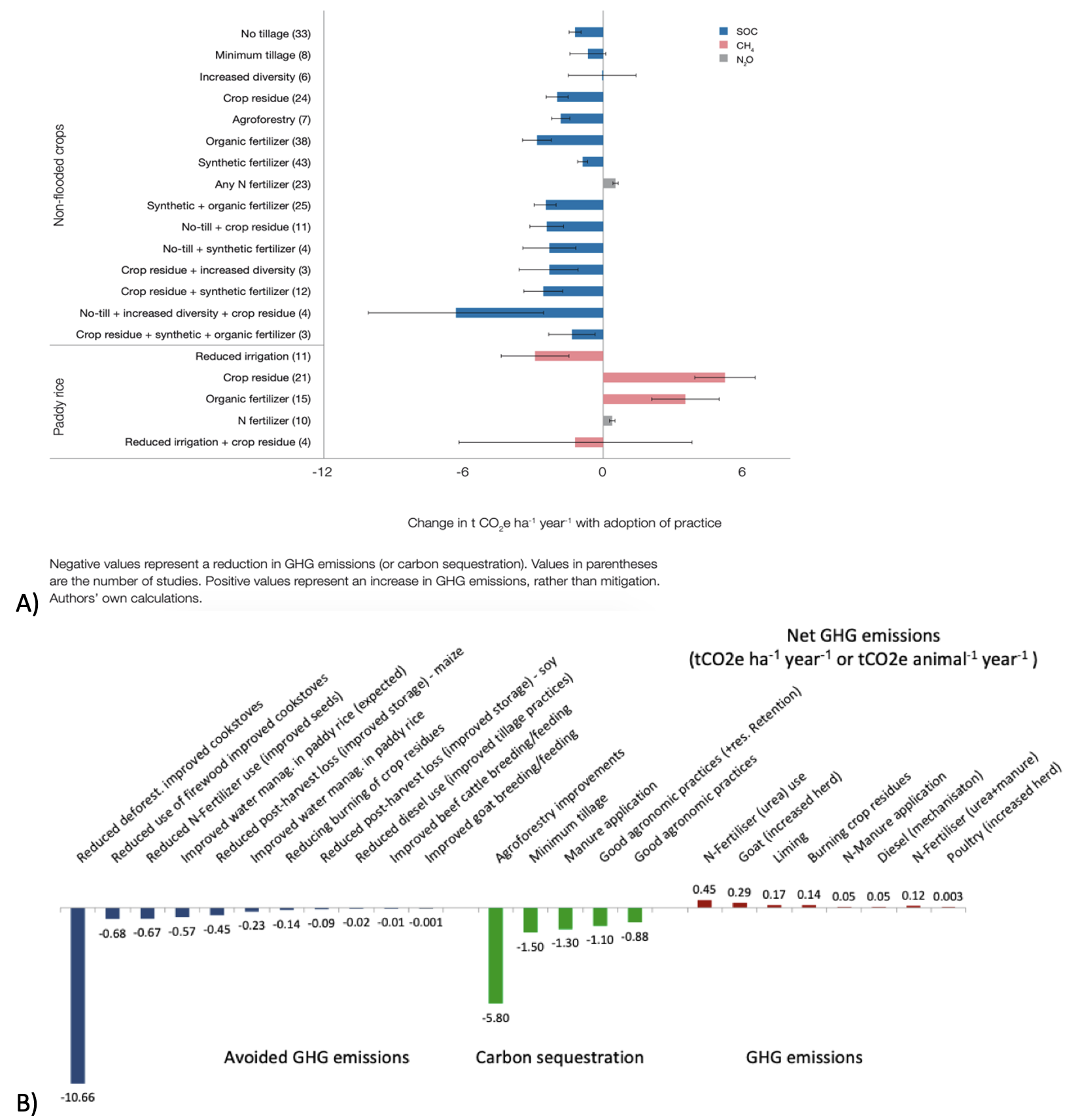
Figure 14. Mitigation potential of agricultural practices promoted by development programs. A) mitigation potential of climate-smart practices; B) the impact of major current and expected agricultural interventions and practices on GHG emissions and carbon sequestration, on an area and animal basis, supported by DfID’s program in countries in Africa and Asia. Source: (a) IFAD (Richards et. al. 2019); (b) DfID (Costa Jr. et al. 2020).

Climate change mitigation is any action that reduces future global climate change. In agriculture, mitigation occurs primarily through reducing emissions, avoiding emissions, or increasing carbon sequestration. While GHG emissions have been understood to be the primary driver of global climate change, managing other drivers such as the albedo of land cover (Carrer 2018, Cardinal 2020), black carbon (Shindell et al. 2011), water cycles, and energy balance (Myhre et al. 2018), or aerosols and volatile organic compounds can also play a role in mitigation.

Mitigation is also referred to as a GHG emissions reduction, abatement, or a change in emissions flux.

To reduce GHGs in a way that matters for the climate, reducing the global amount of GHGs is necessary. This means that even when one entity (country, project, company, farmer) reduces emissions, if others do not, mitigation at the global scale has not occurred.

Reduced emissions can be measured as a reduction in emissions per hectare per time period (usually annually), per unit food product or lifecycle stage. Mitigation is assessed relative to a base year, base period, or future baseline trend. Greenhouse gas footprints can be compared for a practice, farm, supply chain, food product, company, or other entity to show emissions levels; however, to mitigate climate change, a reduction in relation to previous emissions or avoided future emissions is needed.

Avoided emissions are the mitigation expected to occur in the future, i.e. reduction of net emissions relative to a future baseline trend (Figure 1). Avoided emissions are used to describe emissions avoided due to conservation of peatland, forest conservation, efficient use of fertilizer, or more efficient livestock production. Avoided emissions is a critical concept in low-emissions development, where growth in economic or other activity for human health and well-being is necessary and will likely increase emissions. Increasing the GHG emissions-efficiency of food production is one of the simplest routes to avoid future GHG emissions.

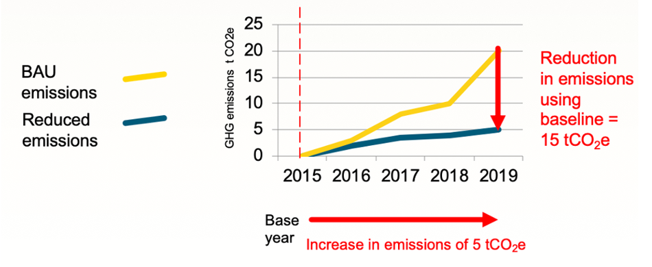
Figure 11. Comparison of use of base year and baseline greenhouse emissions to determine a change in emissions. A baseline is a projection into the future showing business-as-usual (BAU) emissions. A base year is a period before the start of an intervention or period of observation. The example shows a reduction in future emissions (“avoided emissions”), but an increase in emissions relative to the base year. Also, see Calculating Baseline Emissions.

Carbon sequestration is measured as a reduction in emissions or avoided emissions if sequestered carbon is maintained in the face of threats to its loss, such as protecting trees on farms. Unlike the mitigation of GHG emissions, where reductions can be repeated year after year under the same intervention (e.g. more efficient nitrogen use), the amount of carbon sequestration is finite over time. Trees only produce a certain amount of biomass and soils hold a certain amount of carbon. Carbon sequestration is often expressed as an average amount of carbon sequestered per year over a set time period, which by IPCC guidance convention is 20 years, but can also be set according to the length of a project or finance period.

Carbon sequestration can be summed with emissions to produce a net emissions reduction figure; however, net reduction figures should always be disaggregated to reflect mitigation due to emissions and due to carbon sequestration to enable accounting for their different impacts over time. While studies have been done on current stocks of carbon in the soil, biomass on farms, or agroforestry, accounting for changes in carbon sequestration in agriculture has been less common and is a rapidly evolving field (Sanderman et al. 2017; Zomer et al. 2016, Rosenstock et al. 2019).

See LED Options for examples of mitigation in agriculture.

About 82% of agricultural emissions come from low- and middle-income countries (LMIC) (FAOSTAT 2021) and agricultural emissions are expected to grow most rapidly in these countries to meet future increases in food demand and meat consumption. About one-third of agricultural emissions come from only three countries: China, India, and Brazil (Figure 12 and 13).
While emissions per hectare are often low in lower-income countries compared to farms in wealthier countries, the larger extent of farm activity in developing countries contributes to the high proportion of global emissions.

To meet global targets, scenarios suggest mitigation will be needed in most countries around the world, including low and middle-income countries (Kleinwechter et al. 2015) and cost-effective mitigation is possible. However strong arguments also exist for farmers in low- and middle-income countries to not mitigate, including:

• Per capita emissions of poorer farmers tend to be low due to their use of low-intensity agriculture requiring few inputs;
• Principles of low historical responsibility for emissions or low capability or resources to promote new technical practices to reduce emissions (Richards et al. 2017);
• Lower-income farmers are more likely to lack incentives to change practices for environmental goals such as reducing climate change;
• Policymakers want to prioritize food security in vulnerable regions over longer-term environmental goals; and
• Consumers in wealthy countries are often driving emissions in poorer countries. International trade, especially in beef and oilseeds, drives an estimated 29 to 39% of emissions (Pendrill et al. 2019). Emissions are accounted for only at the production stage, thereby masking the impacts of trade.

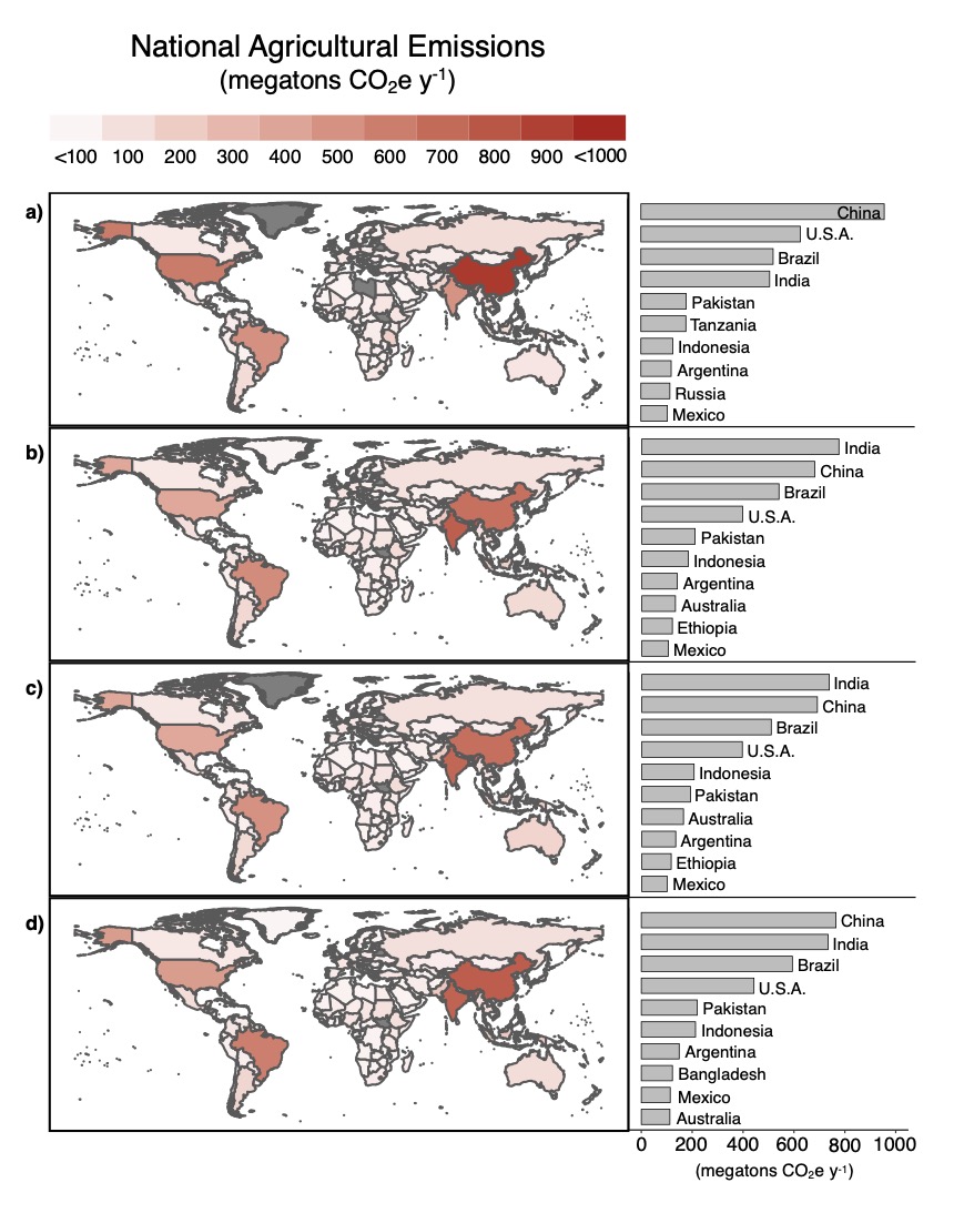
Figure 12. Annual national agricultural emissions (left) and associated top 10 emitters (right) converted to CO2e for (a) UNFCCC, (b) FAOSTAT, (c) WRI-CAIT and (d) EDGAR GHG inventories. UNFCCC data and inventory compilation were obtained via the most recent country-reported National Communication (NC) submitted to the UNFCCC. Grey countries = no NC or data.” Source: (Dittmer, in review).

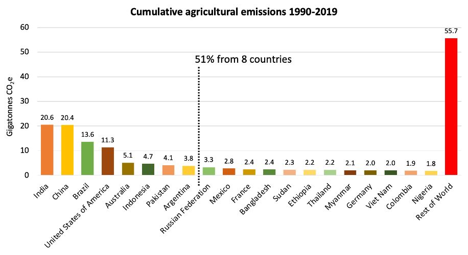
Figure 13. Cumulative emissions by country from the agriculture sector (1990- 2019) (data from FAOSTAT 2019).

Agricultural production and food systems are significant sources of GHG emissions. Crop and livestock production directly contribute 9-14% of global emissions, and the food system as a whole contributes about one-third of global emissions (see Significance of agricultural GHG emissions relative to other sectors below).

Mitigating agricultural emissions and sequestering carbon is also likely necessary to meet the policy targets of the Paris Agreement since research has shown emissions reductions in other sectors alone will be insufficient (see Necessity of mitigation in agriculture to meet global policy targets below).

It is also feasible to reduce emissions in ways that achieve food security and are consistent with the UN Sustainable Development Goals (SDGs). Low-emissions agricultural development is an approach to mitigation that recognizes the need to achieve food security and other development aims in low- and middle-income countries but in ways that also minimize GHG emissions (see Compatibility of low-emission agriculture with the SDGs below).

Globally

Agricultural GHG emissions are about half of the emissions from electricity and heat, which have been the largest contributors to global emissions on average over the last two decades. Over the same time period, agricultural emissions have been higher than the emissions from industry, buildings, waste, or aviation and shipping, while roughly comparable to transport, manufacturing, and construction (Figure 1). When combined with land-use change, for which agriculture is a major driver, agricultural production is the second-largest source of emissions after energy.

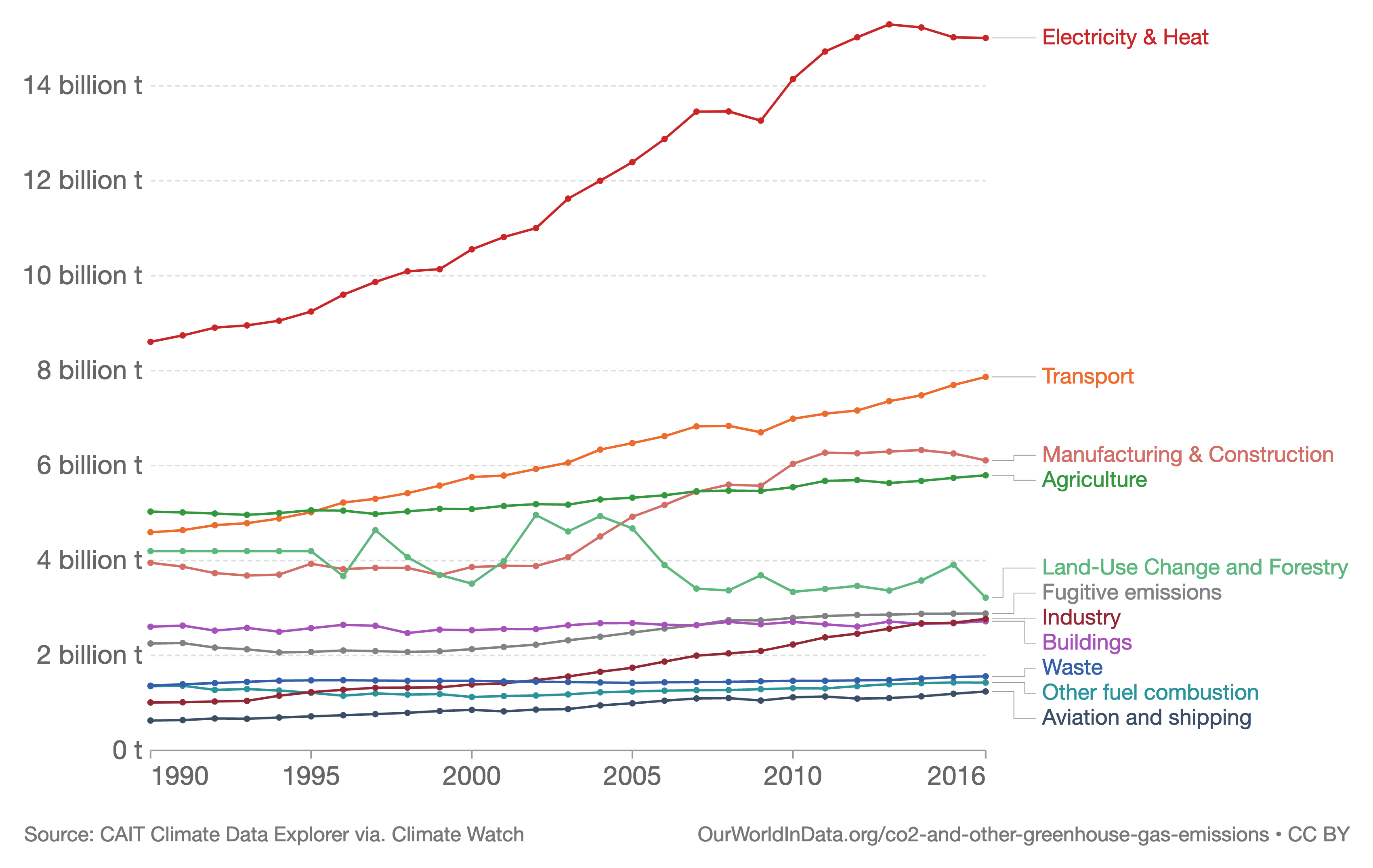
Figure 1. Global greenhouse gas emissions by sector. GHG emissions are measures in tons of carbon dioxide equivalents (CO₂e). Source: Our World in Data, Ritchie and Roser nd.

Nationally

At the national level, agriculture is also a major source of emissions for many countries. On average, agricultural non-CO₂ emissions (methane and nitrous oxide) contributed 19% of countries’ gross national GHG emissions. For non-Annex I countries (predominantly low- and middle-income countries), the average was 21% and 12% for Annex I countries (high-income countries) (Dittmer et al. in review). Seventeen countries reported more than half of their national emissions as coming from agriculture, all of which were non-Annex I countries. Agriculture is typically a larger proportion of the economy in low- and middle-income economies.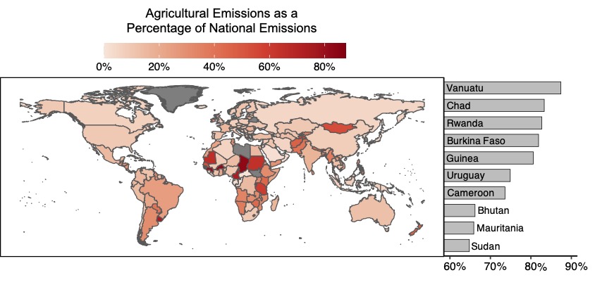

Figure 2. Percent of national emissions from agriculture. Grey countries = no data. Source: Dittmer et al. in review

The 2015 Paris Agreement of the UNFCCC aims:

“… to hold the increase in the global average temperature to well below 2 °C above pre-industrial levels and pursuing efforts to limit the temperature increase to 1.5 °C above pre-industrial levels, recognizing that this would significantly reduce the risks and impacts of climate change” (Article 2).

Scenarios indicate that food system emissions will consume most of the emissions budget needed to meet the 1.5 ˚ or 2 °C goals (Figure 3) (Clark et al. 2020). Agriculture is expected to be the largest source of future surplus emissions as the energy sector is decarbonized with crop and livestock production consuming about 70% of the 21 billion ton CO₂e budget available across all sectors by 2050 if no mitigation action is taken (Searchinger et al. 2019; Bajzelj et al. 2014; Gernaat et al. 2015) (Figure 4).

Figure 3. Food system emissions comprise the majority of future carbon budgets. Shown in this figure are estimates of cumulative GHGH emissions from food production from 2020-20100 based on population, dietary and agricultural trends in a business-as-usual scenario. This is shown relative to total cumulative emissions to keep global average temperature rise below 1.5 ° or 2 °C by 20100. Source Clark et al. 2020 and Our World in Data

According to the IPCC’s 2018 Special Report on the 1.5 °C target, the carbon budget for a likely chance (66% probability) of not exceeding 1.5 °C is 420 GtCO₂, equal to 10 years of annual emissions at the time. To achieve 1.5 °C, all sectors will need to reduce emissions and negative emissions will be needed to offset emissions. In agriculture, models suggest that by 2050, several million square kilometers of pasture (0.5–11 million km²) and non-pasture agricultural lands (4 million km²) will need to be converted to energy crops and forests compared to 2010 if targets are to be met. The agriculture, forestry and land use (AFOLU) sector should be limited to net emissions of no more than 1-11 GtCO₂e/yr (Figure 2).

Agriculture can also sequester carbon or produce “negative emissions.” Increasing the sequestration of carbon in new biomass such as agroforestry or through increased soil organic matter in the soil could provide important means for reaching climate targets.

Reducing livestock emissions, in particular, will be necessary to achieve the 1.5 °C target (Frank et al. 2018), particularly methane. Methane’s short atmospheric lifetime and high global warming potential (GWP) mean that it has a larger impact in the short term (See Global Warming Potential below). Agriculture contributes about half of global anthropogenic methane (Smith et al. 2007)

Reductions in other sectors alone therefore will not be enough to achieve the 2 °C or 1.5 °C policy targets, making mitigation of GHG emissions in agriculture critical to achieving the Paris Agreement.

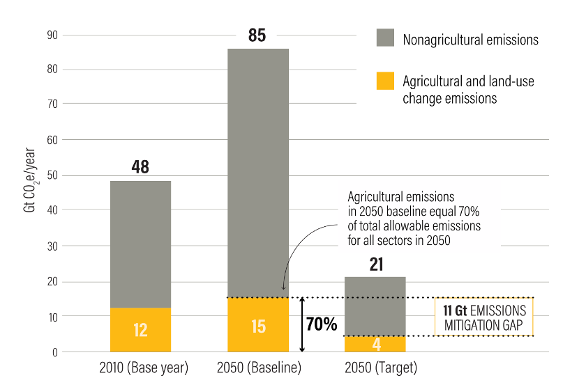
Figure 4. Agricultural emissions as a proportion of targeted emissions for all sectors by 2050. Figures include land-use change due to agriculture. Source: WRI Scope Challenge. See also Frank et al. 2018

Many mitigation practices exist and are already viewed as good agricultural practice regardless of their role in climate change mitigation. Many also contribute to the SDG, hence the possibility of “low-emissions development.”

For example:

• Improved feed for cattle increases productivity (SDG 1, SDG 2) while reducing methane emissions per kg meat or dairy (SDG 13).
• Intermittent drainage of water in paddy rice helps reduce water scarcity (SDG 6) while reducing methane emissions due to flooding (SDG 13).
• Improving soil organic matter contributes to soil productivity for increased farm productivity (SDG 1, SDG 2) and biodiversity (SDG 15) while sequestering carbon (SDG 13)

See also LED Technical Options for reducing emissions.

The greenhouse gases (GHGs) emitted in agriculture are primarily methane (CH₄), nitrous oxide (N₂O), and carbon dioxide (CO₂). Plant biomass and soil organic matter can sequester carbon. Fine particles or droplets of water from land use (aerosols) and surface reflectivity (albedo) influence atmospheric warming to a lesser extent and are less well studied (Smith et al. 2007). Understanding agriculture as part of a dynamic landscape that includes forests, unmanaged lands, and land-use change is essential to projecting future emissions and their mitigation, as well as climate impacts at local, regional and global levels (Figure 5).

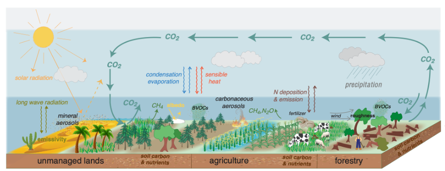
Figure 5. Land-based emissions and impacts on the climate. (Source: Shukla et al. 2019)

Land surface characteristics such as albedo and emissivity determine the amount of solar and long-wave radiation absorbed by land and reflected or emitted to the atmosphere. Surface roughness influences turbulent exchanges of momentum, energy, water, and biogeochemical tracers. Land ecosystems modulate the atmospheric composition through emissions and removals of many GHGs and precursors of SLCFs, including biogenic volatile organic compounds (BVOCs) and mineral dust. Atmospheric aerosols formed from these precursors affect regional climate by altering the amounts of precipitation and radiation reaching land surfaces through their role in cloud physics.

Agriculture can refer to crop or livestock production, farm or pasture land, land-use change due to agriculture, or agricultural supply chains. Defining agricultural emissions precisely in terms of what is included or excluded can help avoid confusion due to differences in scope. In this guidance, the term agricultural emissions refer to the GHG emissions associated with production on farms and pastures, unless otherwise specified.

The scope of agriculture in IPCC guidelines for countries’ reporting to the UNFCCC is formally only the non-CO₂ gases associated with crop and livestock production. Carbon dioxide gases and sequestration are accounted for under land use and land-use change rather than agriculture. Supply chain emissions are usually energy-related and accounted for under transport and industrial emissions. See MRV Systems.

GHG emissions refer to the sum of GHG emissions and carbon sequestration, or what is sometimes called negative emissions (Fuss et al. 2018).

Agricultural GHG emissions are commonly expressed in grams or tons of carbon dioxide equivalent (e.g., GtCO₂e) per hectare or kilogram/liter of product. Emissions per hectare are commonly used to add up or compare emissions for a given area of land. Emissions per unit product are used to show the GHG efficiency of a food product or supply chain. GHG efficiency is also called emissions intensity or yield-scaled emissions.

Methane, nitrous oxide, and carbon dioxide differ in the potency of their warming impact. To reflect these differences, gases are weighted by their global warming potential (GWP), an index reflecting the potency of the gas; GHG emissions from different gases can then be expressed as tons of carbon dioxide equivalents (CO₂e, CO₂eq, or CO₂-e). Using carbon dioxide equivalents enables comparison, trade-off analysis, and aggregation across different gases. However, carbon dioxide equivalents do not reflect well the differences in atmospheric lifetime and roles that gases play in warming the climate (Costa Jr. et al. 2021). For example, methane’s shorter lifetime means that it has much higher impacts—both when it increases or decreases—in the short term compared to carbon dioxide and even nitrous oxide.

Summary of key statistics

• Agriculture directly contributed 9-14% of global emissions, 6.2 ± 1.4 billion tons of CO₂e per year from 2007 to 2016. Agricultural emissions include only methane and nitrous oxide (Jia et al. 2019).
• Agriculture including land-use conversion contributed 14-28% of global emissions, 11.1 ± 2.9 billion tons of CO₂e per year (Mbow et al. 2019).
• Agricultural emissions are expected to increase by (estimates vary by source)
  • 8% by 2020 and 18% by 2050, relative to 2018 (FAOSTAT 2021)
  • 30–40% by 2050 relative to 2007-2016 (Shukla et al. 2019).
• Food systems contributed (estimates vary by source)
  • About one-third of global GHG emissions, or 16 billion tons of CO₂e, annually (1990-2018) (Tubiello et al. 2021).
  • About 21-37% of global GHG emissions, or between 10.8 and 19.1 billion tons of CO₂e, annually (2007-2016) (Shukla et al. 2019).
• Agriculture and agriculture-related land-use change emissions were the major sources of emissions (65-86%) in global food systems (see Table 1).
• 80% of global food systems emissions came from Non-Annex I countries in 2018 (Tubiello et al. 2021).
• The contribution of food systems to national emissions varied from 14-92% per country in 2015 (Crippa 2021).
• Emissions along the supply chain, mostly CO₂ from energy use, contributed 5-10% of global emissions (2007-2016) (Mbow et al. 2019).
• About 6% of global emissions can be attributed to food waste (Poore and Nemecek, 2018).

Agricultural Emissions

Agriculture contributed 6.2 ± 1.4 billion tons of CO₂e per year for the ten-year period 2007 to 2016 or constituted 9-14% of global emissions (Shukla et al. 2019, 2019 IPCC Special Report on Climate Change and Land). The figures for agriculture reflect only the emissions from the non-CO₂ gases nitrous oxide and methane, following IPCC guidance on national GHG accounting.

If related land-use conversion is included, which includes carbon dioxide emissions from biomass and soil, the sector contributed 11.1 ± 2.9 billion tons of CO₂e per year or 14-28% of global emissions.

Land-use conversion for agriculture is the major driver of deforestation, contributing at least 61% (Curtis et al. 2018) and as much as 80% of deforestation-related emissions (Kissinger et al. 2012). About 27% of forest loss due to agriculture (Curtis et al. 2018) can be attributed to agricultural commodities such as beef, cocoa, palm oil, rubber, and soy (Newton et al. 2016).

Agricultural emissions have increased from 2000 to 2010 when estimates suggested 5.0–5.8 billion tons of CO₂e per year (GtCO₂e/yr) (Smith et al. 2014). In the coming decades, agricultural emissions are expected to further increase due to population growth and food security needs, especially in low- and middle-income countries. Estimates vary from an additional 8% by 2020 and 18% by 2050, relative to 2018 (FAOSTAT 2021), to an increase of 30–40% by 2050 relative to 2007-2016 (Shukla et al. 2019).

FAOSTAT is an easy-to-use resource for identifying agricultural emissions by country or region and by year. See also Emissions Data Sources.

The figures reported for global agricultural emissions vary depending on (1) whether accounting includes land conversion due to agriculture or supply chain emissions, (2) the quality and comprehensiveness of activity data used (See Emissions Data Sources), and (3) the time period covered. Care is needed in distinguishing the emissions of food products from farm products. Accounting for the emissions from food (e.g., beef) uses a lifecycle approach, which typically considers emissions from production inputs and the supply chain, in contrast to the emissions for agricultural products (e.g., cattle), which takes a field-emissions approach (See MRV Systems).

Sources of agricultural emissions

The major sources of agricultural GHG emissions of nitrous oxide and methane are livestock, fertilizer use, paddy rice, and open burning (Figure 6). Livestock contributes most of these emissions, with emissions’ impacts equivalent to three times those from aviation (Figure 7). alone comprises 40% of agricultural emissions. Soil and biomass carbon emissions are also dominant sources of anthropogenic CO₂ emissions associated with agriculture, accounted for under land use and land-use change according to IPCC guidance.

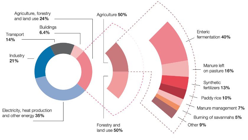
Figure 6. Agriculture and land use currently contribute about 24% of global GHG emissions; about half of that (12%) is from agriculture and the other half from other land use. Source: Richards et al. 2019, citing CDP 2015

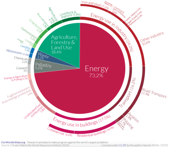
Figure 7. GHG emissions by sector for 2016 (GHG emissions were 49.4 billion tons of CO₂e). Source: Our World in Data and Ritchie and Roser nd

Food Systems

Food systems contributed about one-third of global GHG emissions or 16 billion tons of CO₂e emissions annually for the period 1990-2018 (Tubiello et al. 2021). Food systems emissions historically have been underestimated in official UNFCCC statistics by omitting significant emissions sources such as on-farm energy use, domestic food transport, and food waste disposal (Tubiello et al. 2021, Rosenzweig et al 2021).

Some key figures:

• The major sources of food system emissions globally are agriculture (65%) and agriculture-related land-use change emissions (19%) (Tubiello et al. 2021).
• Eighty percent of global food systems emissions came from Non-Annex 1 countries in 2018 (Tubiello et al. 2021).
• Global per capita emissions from food systems decreased from 2.9 to 2.2 tons CO₂e from 1990 to 2018; per capita emissions in Annex I countries were twice that of Non-Annex I countries in 2018 (Tubiello et al. 2021).
• Pre- and post-agricultural emissions were a larger source in high-income countries compared to low- and middle-income counties. Energy use, industrial activities, and waste management have become larger proportions of emissions over time and in high-income countries, and land-use change emissions smaller (Crippa et al. 2021, (Tubiello et al. 2021).
• The contribution of food systems to national emissions varied from 14-92% per country in 2015 (Crippa et al. 2021).

Estimates of food system emissions vary substantially in the literature, from 9-22 GtCO₂e (Table 1). The main differences in estimates can be attributed to different scopes of accounting, assumptions about agriculture’s contribution to land-use change, sources of activity data, choice of emission factors, and reference time periods. For example, land-use change emissions range from 3 GtCO₂e/yr (19% of food system emissions) (Tubiello et al. 2021) to 5.7 GtCO₂e/yr (32% of food system emissions) (Crippa et al. 2021). Studies also varied in terms of the types of pre-production, retail and post-retail activities, and food waste management included and whether cotton, wool, leather, and biofuels, were counted in the food system (Figure 8) (Ritchie 2018). Some studies calculated their figures by compiling existing knowledge in the literature (Vermeulen et al. 2012; Poore and Nemecek, 2018), while others constructed estimates with coherent sets of underlying data and assumptions.

Most studies used global warming potentials from the IPCC Fifth Assessment report (See Global Warming Potential below) and FAOSTAT activity data to characterize agricultural emissions.

Table 1. Comparison of estimates of food system GHG emissions

Reference	Annual emissions GtCO2e	Reference time period	% from agriculture and related land use
Tubiello et al. (2021)	16	1990-2018	65%
Crippa et al. (2021)	14-22	2015	71%
IPCC report on Climate Change and Land (2019) Mbow et al. 2020. Food security Ch 5 (Table 5.4), Jia et al. 2020. Land-climate interactions Ch 2 (Table 2.2) Shukla et al. Technical Report (p.58)	10.8–19.1	2007–2016	75%
Poore & Nemecek (2018)	13.7	2000–June 2016	59%
Vermeulen et al. (2012)	9.8–16.9	2008, drawing on data from 2004–2008	80%–86%
Rosenzweig et al (2020)	10.8–19.1	2007–2016	See IPCC Land Report 2019
Clark et al. (2020)	16.96 (1,356 over 80 years)	2020–2100	No figure

Food products can be ranked according to their emissions. Beef has had the highest level of emissions whereas root crops and horticultural trees are among the lowest (Figure 9). Emissions along the supply chain, mostly CO₂ from energy use, contribute 5-10% of global emissions (Mbow et al. 2019). About 6% of global emissions can be attributed to food waste (Poore and Nemecek, 2018).

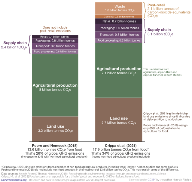
Figure 8. How much GHG emissions come from food systems. Source: Our World in Data

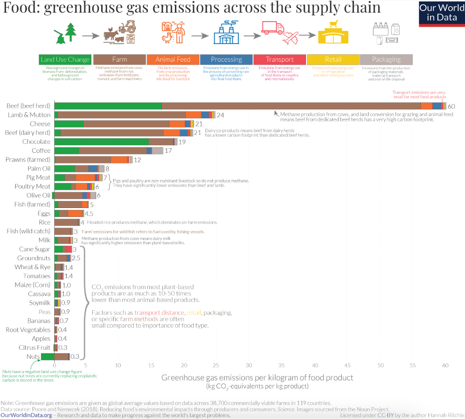
Figure 9. GHG emissions by food products across the supply chain. Source: Our World In Data (Poore and Nemecek, 2018).

Global warming potential (GWP) describes the potential impact of a given gas on atmospheric warming or, that is, energy from the sun that is not absorbed by the earth and radiates back to space. The IPCC (1996) defines GWP as the “cumulative radiative forcing, both direct and indirect effects, over a specified time horizon resulting from the emission of a unit mass of gas related to some reference gas. Carbon dioxide (CO₂) is the standard reference gas.”

The most widespread climate warming metric in use today is GWP 100, or GWP₁₀₀. GWP₁₀₀ is the amount of energy one ton of a gas will absorb over 100 years.

GWP allows the comparison of different GHGs on global climate impacts. The larger the GWP, the larger the climate impact.

Methane (CH₄), nitrous oxide (N₂O), and CO₂ differ in the potency of their impact on the climate. Over a 100-year time frame, methane is 28 times more potent and nitrous oxide 265 times more potent than carbon dioxide (Figure 6). Carbon dioxide is used by convention as the reference point, so the GWP is 1 for CO₂.

Gases’ differential impacts on the atmosphere depend mostly on their atmospheric lifetime, which reflects their chemical reactiveness and decay mechanisms. Methane is a short-lived climate pollutant, lasting only about 12 years. Nitrous oxide lasts about 116 years (Prather et al. 2015) and is considered a long-lived pollutant. Carbon dioxide is also considered a long-lived pollutant but does not have a single atmospheric lifetime, due to multiple sources of CO₂ uptake and removal from and re-release to the atmosphere (e.g., plants, oceans) (Archer et al. 2008). While CO₂ levels may peak in less than 300 years, the impacts of CO₂ can persist for several millennia (Archer et al. 2008, Solomon et al. 2008). Archer et al. 2008 predict atmospheric CO₂ remnant ranges of 10-30% at 10,000 years and 14-60% at 1000 years.

GWP values are published by the IPCC. The most recent GWP values from the IPCC 6th Assessment Report indicate a GWP value of 27.2 and 273 for non-fossil fuel CH₄ and N₂O, respectively (Table 2) (2021, see Chapter 7, Table 7.15). Estimates are updated regularly to reflect the best evidence available and the IPCC has published three sets of GWP values since its Second Assessment report in 1995. Earlier calculations of emissions may therefore reflect outdated values. (Table 3).

Radiative forcing of the earth’s atmosphere due to greenhouse gas emissions is the change in net (down minus up) irradiance in watts per square meter. Radiative forcing describes the significance of GHG emissions’ impacts for warming of the climate but does not describe actual warming impacts due to other feedback mechanisms (general circulation models of the climate are more appropriate for understanding warming impacts). (Forster et al. 2007)

Table 2. Emission metrics for agricultural greenhouse gases expressed as global warming potential over 20, 100, or 500 years. (Source Forster et al. 2021).

Greenhouse gas	Lifetime (years)		GWP-20		GWP-100		GWP-500
	value	± error	value	± error	value	± error	value	± error
CO2	Multiple		1		1,000		1,000
CH4-fossil	11.8	1.8	82.5	25.8	29.8	11	10.0	3.8
CH4-non fossil	11.8	1.8	80.8	25.8	27.2	11	7.3	3.8
N2O	109	10.0	273	118	273	130	130	64

Table 3. Comparison of GWP values for agricultural greenhouse gases from different IPCC reports (Source: Adapted from WRI and Forster et al. 2021).

GHG	GWP values for 100-year time horizon
	IPCC Second assessment report	IPCC Fourth assessment report	IPCC Fifth assessment report	IPCC Sixth assessment report
CO2	1	1	1	1
CH4	21	25	28	29.8 (fossil fuel) 27.2 (non-fossil fuel)
N2O	310	298	265	273

GWP for short-lived greenhouse gases

The use of CO₂e units masks the global warming potential of short-lived gases, like CH₄, that reduce in concentration more rapidly over a few decades or less. This means that the CH₄ emitted a century ago no longer exists today. To correct this distortion, GWP* (GWP star) allocates the emissions of each gas according to its actual estimated average atmospheric lifetime rather than the standardized 100-year period.

GWP* is a useful complement to conventional climate metrics such as GWP₁₀₀ because it better reflects the actual warming caused by CH₄ emissions. For example, using GWP₁₀₀, a constant rate of CH₄ emissions appears to have three to four times greater impact on climate warming than actually observed. The use of GWP* can correct this misestimation. See Figure 10 for a comparison of GWP₁₀₀ versus GWP*.

Using GWP*, a steady ~0.35% per annum decline in CH₄ emissions from agriculture from 2020 to 2040 would be sufficient to cause no additional increase in global temperatures from agricultural CH₄ emissions (analogous to the impact of achieving net-zero emissions).

Faster rates of CH₄ emission reduction would reduce the contribution of agricultural methane to a global temperature below current levels (having an analogous impact to removing CO₂ from the atmosphere). A sustained reduction of ~5% p.a. could neutralize the additional warming due to agricultural CH₄ since 1980, bringing its contribution to global temperature increase back to 1980 levels. However, a 1.5% p.a. increase in CH₄ emissions would lead to rapid climate impacts about 1.5 times greater than indicated by GWP₁₀₀ (Costa Jr. et al. 2021).

The application of GWP* suggests that achieving effective climate neutrality, in the sense of no additional warming impact, for CH₄ emissions in agriculture is more attainable than previously understood, further emphasizing the important benefits of making significant cuts in CH₄ emissions immediately.

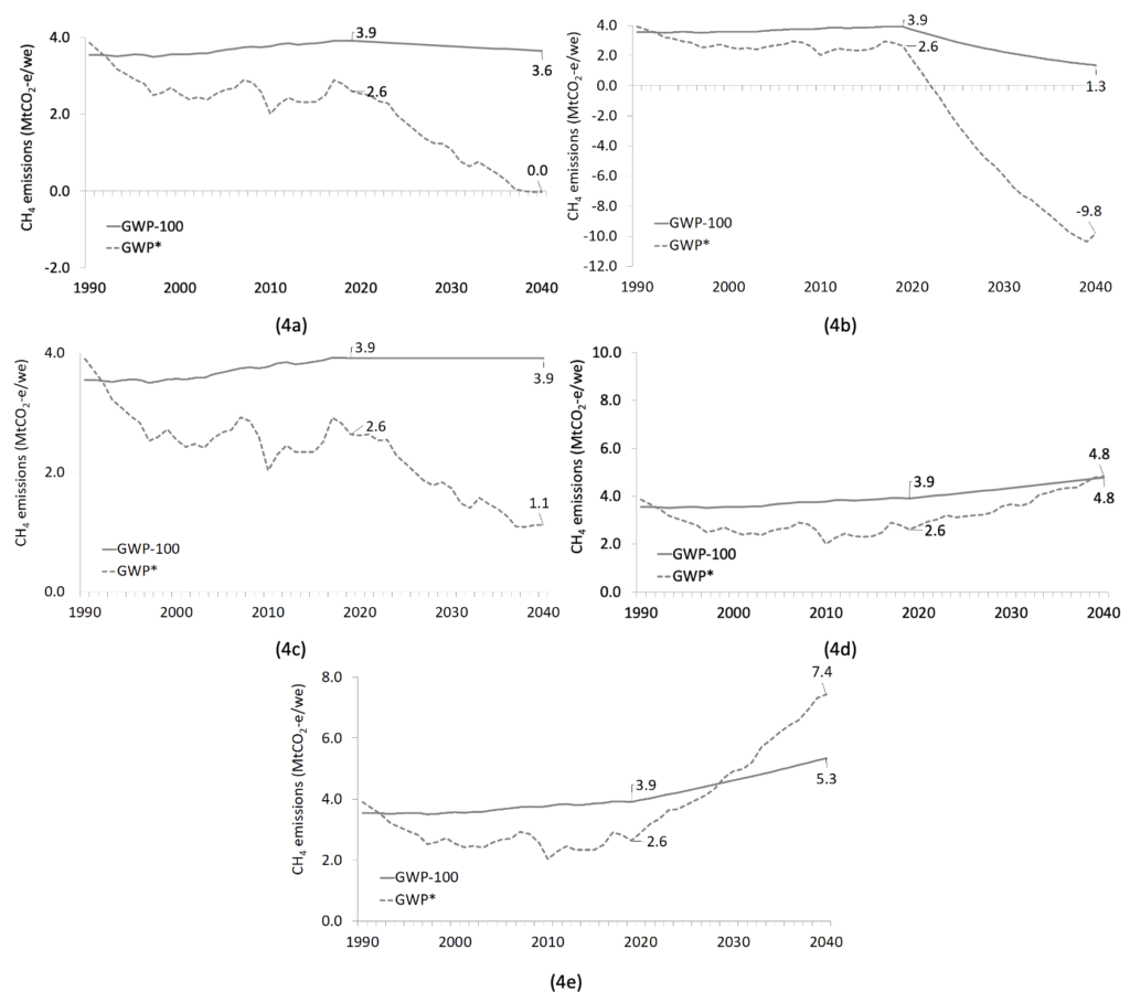
Figure 10. Global agriculture methane (CH₄) emissions from 2020 to 2050 using GWP₁₀₀ (IPCC-AR5) and GWP* accounting methods. Emissions scenarios include CH₄ emissions at reduction of 0.35% p.a. (a), a decrease of 5.00% p.a. (b), a constant rate (0% increase/decrease), and (c) an increase of about 1.00% p.a. (d) and 1.50% p.a. (e).