Jump to: Methods and sources of activity data | Methods and sources of emissions factors
Agroforestry is generally not accounted for in national GHG inventories but can make an important contribution to climate change mitigation (Zomer et al. 2016; Feliciano et al. 2018; Rosenstock et al. 2019). There is no IPCC methodology specific to agroforestry or trees on agricultural land. This section describes the requirements for activity data and emission factors for the general IPCC methodology for measuring changes in biomass carbon stocks and carbon stocks in dead organic matter. It also discusses other approaches used to estimate carbon stock changes associated with agroforestry systems. This overview focuses on agroforestry as a land-use type (land remaining in a land-use category over time) and does not cover land-use change.
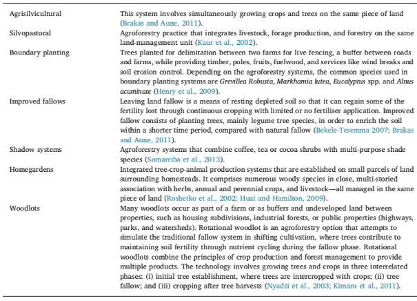
Agroforestry is practiced in many ways, from living fences and home gardens to woodlots and multi-strata agroforestry. Current definitions of agroforestry systems emphasize the roles trees play in integrated eco-system management, connecting trees, forests, farms, livelihoods, landscapes and governance (van Noordwijk et al. 2016). Historically, however, narrower definitions focused tightly on trees planted or intentionally managed on croplands and rangelands (Nair and Nair 2003). Common typologies of agroforestry systems include agrisilviculture, silvopastoral, boundary planting, improved fallows, shadows systems, home gardens and woodlots (Feliciano et al. 2018).
Definition of some common agroforestry systems (Feliciano et al. 2018):
What data are required?
Carbon stock changes within a stratum (or subdivision of land area) are estimated by adding up changes in 5 carbon pools. Harvested wood products are considered an additional pool.

- ΔCLUi = carbon stock changes for a stratum of a land-use category
- Subscripts denote the following carbon pools:
- AB = above-ground biomass
- BB = below-ground biomass
- DW = deadwood
- LI = litter
- SO = soils
- HWP = harvested wood products
Tier 1 methods make several assumptions that simplify the approach:
- ΔCBB is assumed to be zero.
- Deadwood and litter pools are lumped together as “dead organic matter” and assumed to be zero for non-forest land-use categories. The change in dead organic matter is also assumed to be zero for land remaining in the same land use category, on the basis that the average transfer rate into dead organic matter (deadwood and litter) is generally equal to the average transfer rate out of dead organic matter.
There are two general methods for estimating changes in any given carbon pool: the gain-loss method and the stock-difference method.
Grain-loss method
![]()
- ΔC = annual carbon stock change in the pool (ΔCAB, ΔCAB, etc.), tonnes C yr-1
- ΔCG = annual gain of carbon, tons C yr-1
- ΔCL = annual loss of carbon, tons C yr-1
The gain-loss method lends itself well to modeling approaches using empirically-derived coefficients. But the stock-difference method (below) is equally valid.
For changes in biomass carbon stocks (ΔCAB, ΔCBB), ∆CG = annual increase in carbon stocks due to biomass growth for each land sub-category, and ∆CL = annual decrease in carbon stocks due to biomass loss for each land sub-category, both in units of tonnes C yr-1.
∆CG is calculated by multiplying the area of land by mean annual biomass growth and the carbon fraction of dry matter:

- ∆CG = annual increase in biomass carbon stocks due to biomass growth in land remaining in the same land-use category by vegetation type and climatic zone, ton C yr-1
- A = area of land remaining in the same land-use category, ha
- GTOTAL= mean annual biomass growth, ton d. m. ha-1 yr-1
- i = ecological zone (i = 1 to n)
- j = climate domain (j = 1 to m)
- CF = carbon fraction of dry matter, ton C (ton d.m.)-1
GTOTAL is calculated differently depending on whether a Tier 1 or Tier 2/3 method is used:
Tier 1

- GW = average annual above-ground biomass growth for a specific woody vegetation type, tons d. m. ha-1 yr-1
- R = ratio of below-ground biomass to above-ground biomass for a specific vegetation type, in ton d.m. below-ground biomass (ton d.m. above-ground biomass)-1. R must be set to zero if assuming no changes of below-ground biomass allocation patterns (Tier 1).
If using the Tier 1 method, default values of Gw may be used (Tables 4.9, 4.10 and 4.12; Chapter 4; IPCC, 2019)
Tier 2 or 3

- GW = average annual above-ground biomass growth for a specific woody vegetation type, tonnes d. m. ha-1 yr-1
- R = ratio of below-ground biomass to above-ground biomass for a specific vegetation type, in tonne d.m. below-ground biomass (tonne d.m. above-ground biomass)-1. R must be set to zero if assuming no changes of below-ground biomass allocation patterns (Tier 1).
- IV = average net annual increment for specific vegetation type, m3 ha-1 yr-1
- BCEFI = biomass conversion and expansion factor for converting merchantable volume to total above-ground biomass growth for specific vegetation type, tonnes above-ground biomass growth (m3 net annual increment)-1
BCEFI can be calculated:

Stock-difference method

- ΔC = annual carbon stock change in the pool, tons C yr-1
- Ct1 = carbon stock in the pool at time t1, tons C
- Ct2 = carbon stock in the pool at time t2, tons C
Suppose the C stock changes are estimated on a per hectare basis; in that case, the value is multiplied by the total area within each stratum to obtain the total stock change estimate for the pool.
The stock-difference method requires that countries measure the stocks of different biomass pools in forests and other land uses at periodic intervals. This method requires greater resources and is suitable to countries adopting a Tier 3, and sometimes a Tier 2 approach, but may not be suitable for countries using a Tier 1 approach due to data limitations.
When estimating changes in biomass carbon stocks using the stock-difference method, Ct1 and Ct2 = the total carbon in biomass for each land sub-category at times t1 and t2, respectively, in tons C. Ct1 and Ct2 are calculated using the following equation:

- A = area of land remaining in the same land-use category, ha
- V = merchantable growing stock volume, m3 ha-1
- i = ecological zone i (i = 1 to n)
- j = climate domain j (j = 1 to m)
- R = ratio of below-ground biomass to above-ground biomass, tonne d.m. below-ground biomass (tonne d.m. above-ground biomass)-1
- CF = carbon fraction of dry matter, tonne C (tonne d.m.)-1
- BCEFS = biomass conversion and expansion factor for the expansion of merchantable growing stock volume to above-ground biomass, tonnes above-ground biomass (m3 growing stock volume)-1 (Table 4.5, Chapter 4; IPCC, 2006 – no refinement provided in IPCC, 2019).
Annual biomass carbon gain, ΔCG
Mean above-ground biomass growth (increment), GW
Default values for GW are available (Tables 4.9, 4.10 and 4.12; Chapter 4; IPCC, 2019)
If using the Tier 2/3 method to calculate GW, default values are also available for IV (Tables 4.9, 4.11; Chapter 4; IPCC, 2019) and for BCEFI (Table 4.5, Chapter 4; IPCC, 2006 – no refinement provided in IPCC, 2019).
Separate data on biomass expansion factor for increment (BEFI) and basic wood density (D) can also be used to convert the available data to GW. Tables 4.13 and 4.14 (Chapter 4; IPCC, 2006 – no refinement provided in IPCC, 2019) provide default values for basic wood density.
Annual biomass carbon loss, ΔCL
Methods and sources of activity data
- Zomer R, et al. 2016. Global Tree Cover and Biomass Carbon on Agricultural Land: The contribution of agroforestry to global and national carbon budgets.
- Zomer R, et al. 2014. Trees on farms: an update and reanalysis of agroforestry’s global extent and socio-ecological characteristics.
Methods and sources of stock reference or stock change factors
- Feliciano D, et al. 2018. Which agroforestry options give the greatest soil and above-ground carbon benefits in different world regions?
- Feyisa K, et al. 2018. Allometric equations for predicting above-ground biomass of selected woody species to estimate carbon in East African rangelands.
- Mokria M, et al. 2018. Mixed-species allometric equations and estimation of aboveground biomass and carbon stocks in restoring degraded landscape in northern Ethiopia.
- Kuyah S, et al. 2012a. Allometric equations for estimating biomass in agricultural landscapes: I. Aboveground biomass.
- Kuyah S, et al. 2012b. Allometric equations for estimating biomass in agricultural landscapes: II. Belowground biomass
- Other resources on allometric equations in agroforestry systems: World Agroforestry