Jump to: Methods and sources of activity data | Methods and sources of stock reference or stock change factors
Changes in land use or management can affect soil carbon (C) stocks. Although organic and inorganic forms of C are found in soils, land use and management typically have a larger impact on organic C stocks. Soil C inventories include estimates of soil organic C stock changes for mineral soils and CO2 emissions from organic soils due to enhanced microbial decomposition caused by drainage and associated management activity. In addition, inventories can address C stock changes for soil inorganic C pools (e.g., calcareous grassland that becomes acidified over time) if sufficient information is available to use a Tier 3 approach (see box below). Mineral soils are the typical soils found in agriculture and contain 1-6% organic matter. Organic soils have much higher concentrations, e.g., peat soils contain more than 60% organic matter.
The 2019 Refinement to the 2006 IPCC Guidelines uses six land-use categories: forest land, cropland, grassland, wetlands, settlements, and other land types. This section describes the general approach for estimating soil C stock changes, then goes into further detail for cropland and grassland categories.
| Soil inorganic carbon (SIC) |
|---|
| Soil inorganic carbon (SIC) comprises pedogenic carbonates and bicarbonates, which are particularly abundant in alkaline soils. In soils in which SIC is predominant, quantifying it can render useful ancillary information (FAO, 2019). Quantitative methods for total carbonate determination were described by Loeppert and Suarez (1996). The effects of land-use and management activities on soil inorganic C stocks and fluxes are linked to site hydrology and depend on the specific mineralogy of the soil. Further, accurate estimation of the effects requires following the fate of discharged dissolved inorganic C and base cations from the managed land, at least until they are fully captured in the oceanic inorganic C cycle. No Tier 1 or 2 methods are provided for estimating the change in soil inorganic C stocks due to limited scientific data for derivation of stock change factors; thus the net flux for inorganic C stocks is assumed to be zero. Thus, a comprehensive hydrogeochemical analysis that tracks the fate of dissolved CO2, carbonate and bicarbonate species and base cations (e.g., Ca and Mg) applied to, within, and discharged from, managed land over the long term is needed to accurately estimate net stock changes (IPCC, 2006). |
Estimating soil carbon
What data are required?
Tier 1
The annual change in organic and inorganic carbon stocks in soils in a given land area is calculated using the following general equation. For Tier 1 and 2 methods, soil organic C (SOC) stocks for mineral soils are computed to a default depth of 30 cm. Greater depth can be selected and used for Tier 2 calculations if data are available.

- ∆Csoils = annual change in organic and inorganic carbon stocks in soils, tonnes C yr-1
- ∆Cmineral = annual change in organic carbon stocks in mineral soils, tonnes C yr-1
- Lorganic = annual loss of organic carbon from drained organic soils, tonnes C yr-1
- ΔCinorganic = annual change in inorganic carbon stocks from soils, tonnes C yr-1 (this is assumed to be 0 unless using a Tier 3 approach)
Mineral soils
The Tier 1 method is based on changes in soil C stocks over a finite period of time. The change is computed based on C stock after the management change relative to the carbon stock in a reference condition (i.e., native vegetation that is not degraded or improved). Calculation of soil C stock changes rests on two assumptions:
- Over time, soil organic C reaches a spatially-averaged, stable value specific to the soil, climate, land-use and management practices; and
- SOC stock changes during the transition to a new equilibrium SOC are linear.

- ∆Cmineral = annual change in carbon stocks in mineral soils, tonnes C yr-1
- SOC0 = soil organic carbon stock in the last year of an inventory time period, tonnes C
- SOC(0-T) = soil organic carbon stock at the beginning of the inventory time period, tonnes C
- SOC0 and SOC(0-T) are calculated using the SOC equation where the reference carbon stocks and stock change factors are assigned according to the land-use and management activities and corresponding areas at each of the points in time (time = 0 and time = 0-T)
- T = number of years over a single inventory time period, yr
- D = Time dependence of stock change factors which is the default time period for the transition between equilibrium SOC values, yr. Commonly 20 years, but depends on assumptions made in computing the factors FLU, FMG and FI. If T exceeds D, use the value for T to obtain an annual rate of change over the inventory time period (0-T years).
- c,s,i = c represents climate zones, s represents soil types, and i represents the set of management systems that are present in a country
- SOCREF = the reference carbon stock, tonnes C ha-1 (Table 2.3; IPCC, 2019)
- FLU = stock change factor for land-use systems or sub-system for a particular land-use, dimensionless (Table 5.5; IPCC, 2019 for croplands and Table 6.2; IPCC 2019 for grasslands)
- FMG = stock change factor for management regime, dimensionless (Table 5.5; IPCC, 2019 for croplands and Table 6.2; IPCC 2019 for grasslands)
- FI = stock change factor for input of organic matter, dimensionless (Table 5.5; IPCC, 2019 for croplands and Table 6.2; IPCC 2019 for grasslands)
- A = land area of the stratum being estimated, ha. All land in the stratum should have common biophysical conditions (i.e., climate and soil type) and management history over the inventory time period to be treated as one unit for analysis.
Estimating soil carbon stock changes in mineral soils thus requires data on the land area under each land use and management category in the first year (time 0-T) and last year (time 0) of the inventory time period. IPCC (2006) guidelines recognize three approaches for representing land-use areas.
Approach 1. Represents land areas within a defined spatial unit. Only the net changes in land-use area can be tracked through time. Consequently, the exact location or pattern of the land uses is not known within the spatial unit, and the exact changes in land-use categories cannot be ascertained. This approach does not allow for analysis of soil C stock changes for land remaining within a land use category.
Table 1. Net changes in land use within a defined special unit
| Land use category/strata | Initial land area (million ha) | Final land area (million ha) | Net change in area (million ha) | Notes |
|---|---|---|---|---|
| Forest land | 7 | 8 | 1 | |
| Grassland (unimproved) | 65 | 63 | -2 | Decrease in area indicates land use conversion. Could require further stratification for different management regimes, etc. |
| Grassland (improved) | 19 | 19 | 0 | No land use conversion. Could require further stratification for different management regimes, etc. |
| Cropland (total) | 31 | 29 | -2 | Decrease in area indicates land use conversion. Could require further stratification for different management regimes, etc. |
| Wetlands (total) | 0 | 0 | 0 | |
| Settlements (total) | 5 | 8 | 3 | |
| Total | 127 | 127 | 0 |
Using this approach, changes in mineral soil C stocks are calculated as:

Approach 2 & 3. In contrast, activity data may be collected based on surveys, remote sensing imagery, or other data providing the total areas for each land management system and the specific transitions in land use and management overtime on individual parcels of land. These are considered Approach 2 and 3 activity data in Chapter 3, and soil C stock changes are computed using formulation B of Equation 2.25 (IPCC, 2019):

- p = a parcel of land representing an individual unit of area over which the inventory calculations are performed
Table 2. Illustrative example of approach 2 data in a land-use conversion matrix with category stratification (based on Table 3.5; IPCC, 2019)*
| Final/Initial | Forest land | Grassland (unimproved) | Grassland (improved) | Cropland | Wetlands | Settlements | Final Area |
|---|---|---|---|---|---|---|---|
| Forest land | 5 | 1 | 2 | 1 | 9 | ||
| Grassland (unimproved) | 6 | 61 | 67 | ||||
| Grassland (improved) | 3 | 39 | 42 | ||||
| Cropland | 10 | 4 | 45 | 59 | |||
| Wetlands | 0 | 0 | |||||
| Settlements | 1 | 1 | 5 | 7 | |||
| Final Area | 22 | 69 | 41 | 47 | 0 | 5 | 184 |
| *for approach 3 (uses spatially explicit observations of land-use categories and land-use conversions) data can be summarized in a table similar to the one used for Approach 2, with the difference that the locations of land use and land-use conversions are known. | |||||||
For croplands, IPCC (2006) provides default Tier 1 land-use factors (FLU) for land under long-term cultivation of annual (non-paddy) crops, paddy rice, perennial tree crops, and set aside. Tier 1 management (FMG) and input (FI) factors are also available.
Table 3. Relative carbon stock change factors (FLU, FMG, and Fi) (over 20 years) for management activities on cropland
| Factor | Level | Temperature regime | Moisture regime | IPCC defaults | Error |
|---|---|---|---|---|---|
| Land use (FLU) | Long-term cultivated | Cool Temperate/ Boreal | Dry | 0.77 | ±14% |
| Moist | 0.70 | ±12% | |||
| Warm Temperate | Dry | 0.76 | ±12% | ||
| Moist | 0.69 | ±16% | |||
| Tropical | Dry | 0.92 | ±13% | ||
| Moist/Wet | 0.83 | ±11% | |||
| Paddy rice | All | Dry and Moist/Wet | 1.35 | ±4% | |
| Perennial/Tree crop | Temperate/Boreal | Dry and moist | 0.72 | ±22% | |
| Tropical | Dry and Moist/Wet | 1.01 | ±25% | ||
| Set aside (<20 yrs) | Temperate/Boreal and Tropical | Dry | 0.93 | ±11% | |
| Moist/Wet | 0.82 | ±17% | |||
| Tropical Montane | n/a | 0.88 | ±17% | ||
| Tillage (FMG |
Full | All | Dry and Moist/Wet | 1.00 | n/a |
| Reduced | Cool Temperate/ Boreal | Dry | 0.98 | ±5% | |
| Moist | 1.04 | ±4% | |||
| Warm Temperate | Dry | 0.99 | ±3% | ||
| Moist | 1.05 | ±4% | |||
| Tropical | Dry | 0.99 | ±7% | ||
| Moist/Wet | 1.04 | ±7% | |||
| No-tillage | Cool Temperate/ Boreal | Dry | 1.03 | ±4% | |
| Moist | 1.09 | ±4% | |||
| Warm Temperate | Dry | 1.04 | ±3% | ||
| Moist | 1.10 | ±4% | |||
| Tropical | Dry | 1.04 | ±7% | ||
| Moist/Wet | 1.10 | ±5% | |||
| Input (Fi) | Low | Temperate/Boreal | Dry | 0.95 | ±13% |
| Moist | 0.92 | ±14% | |||
| Tropical | Dry | 0.95 | ±13% | ||
| Moist/ Wet | 0.92 | ±14% | |||
| Tropical montane | n/a | 0.94 | ±50% | ||
| Medium | All | Dry and Moist/ Wet | 1.00 | n/a | |
| High without manure | Tem-perate/ Boreal and Tropical | Dry | 1.04 | ±13% | |
| Moist/ Wet | 1.11 | ±10% | |||
| Tropical montane | n/a | 1.08 | ±50% | ||
| High – with manure | Temperate/ Boreal and Tropical | Dry | 1.37 | ±12% | |
| Moist/ Wet | 1.44 | ±13% | |||
| Tropical montane | n/a | 1.41 | ±50% |
For grasslands, IPCC (2006) uses a single land-use factor (FLU) of 1.0. Management factors (FMG) vary according to the level of degradation or improvement of the grassland. Input factors (FI) are used only for improved, managed grassland.
Table 4. Relative carbon stock change factors (FLU, FMG, and Fi) (over 20 years) for grassland management
| Factor | Level | Temperature regime | Moisture regime | IPCC defaults | Error |
|---|---|---|---|---|---|
| Land use (FLU) | All | All | All | 1.0 | N/A |
| Management (FMG) | Nominally managed (non–degraded) | All | 1.0 | N/A | |
| High Intensity Grazing | All | 0.9 | ±8% | ||
| Severely degraded | All | 0.7 | ±40% | ||
| Improved grassland | Temperate/Boreal | 1.14 | ±11% | ||
| Tropical | 1.17 | ±9% | |||
| Tropical Montane | 1.16 | ±40% | |||
| Input (Fi) | Medium | All | 1.0 | N/A | |
| High | All | 1.11 | ±7% |
Organic soils
The basic methodology for estimating C emissions from organic (e.g., peat-derived) soils is to assign an annual emission factor that estimates C losses following drainage.
![]()
- Lorganic = annual carbon loss from drained organic soils, tonnes C yr-1
- A = land area of drained organic soils in climate type c, ha
- Note: A is the same area (Fos) used to estimate N2O emissions from drained organic soils (above). See Emissions from Managed Soils
- EF = emission factor for climate type c, tonnes C ha-1 yr-1
Therefore, the activity data required to estimate C emissions from organic soils are the area of drained or managed organic soils, categorized by climate (temperate and tropical). In addition, for temperate forest land, areas should be further stratified by soil fertility (nutrient-rich and nutrient-poor). In case no stratification by soil fertility is possible, countries may rely on expert judgment. These data will also be needed to estimate N2O emissions from drained organic soils. IPCC (2006) provides Tier 1 emission factors for drained grassland organic soils and cropland organic soils, found in Table 5 below.
Table 5. Tier 1 emission factors (EFs) for drained grassland and cultivated cropland organic soils
| Climatic temperature regime | IPCC default (tons C ha-1 yr-1) | Error |
|---|---|---|
| Annual EFs for cultivated organic soils (Table 5.6, Chapter 5, IPCC, 2006) | ||
| Boreal/Cool Temperate | 5 | ±90% |
| Warm Temperate | 10 | ±90% |
| Tropical/Sub-Tropical | 20 | ±90% |
| Annual EFs for drained grassland organic soils (Table 6.3, Chapter 6, IPCC, 2006) | ||
| Boreal/Cool Temperate | 0.25 | ±90% |
| Warm Temperate | 2.5 | ±90% |
| Tropical/Sub-Tropical | 5 | ±90% |
Tier 2
Approach 1. Developing Country-Specific Factors for the Default Equations
The Tier 2 method for calculating soil C stocks changes uses the same calculation steps as for Tier 1. Still, it incorporates country-specific data to improve four components of the Tier 1 approach:
- Type of management system: default systems (e.g., improved and unimproved grassland) can be disaggregated into a finer characterization that better represents the impact of management on soil organic C stocks in the land area inventory.
- Climate regions and soil types: more detailed soil and climate classifications, specific to the region or country of the inventory, could be used.
- Reference C stocks: identifying country- or region-specific reference levels of C stocks (SOCref) is another option for improving an inventory of soil C stock changes.
- Stock change factors: country- or region-specific soil C stock change factors developed from measurement data and model simulations.
Approach 2. Steady-State Method
The Tier 2 steady-state method is an intermediate complexity approach between Tier 1 and Tier 3 methods and is based on a steady-state solution to the three-soil organic C sub-pools in the Century ecosystem model. It provides, therefore, an optional alternative method for estimating soil C stock changes in the 0-30 cm layer of mineral soils in Cropland Remaining Cropland.
The Tier 2 steady-state method incorporates spatial and temporal variation in climate, organic carbon inputs to soils, soil properties, and management practices. However, compilers can further develop and/or parameterize this model given appropriate datasets (Tier 3). The method is not appropriate for rice cultivation and is not parameterized to estimate the change in soil organic C stocks due to biochar C amendments.
Table 6. Globally calibrated model parameters to be used to estimate soc changes for mineral soils with the tier 2 steady-state method (Table 5.5a, Chapter 5, IPCC, 2019)
| Parameter | Practice | Value (min, max) | Standard Deviation | Description |
|---|---|---|---|---|
| TillFAC | Full-till | 3.036 (1.4, 4.0) | 0.579 | Tillage disturbance modifier for decay rates |
| Reduced-till | 2.075 (1.0, 3.0) | 0.569 | ||
| No-till | 1 | - | ||
| WS | All | 1.331 (0.8, 2.0) | 0.386 | slope parameter for Mappeti term to estimate Wfac |
| Kfaca | All | 7.4 | n/a | Decay rate constant under optimal conditions for decomposition of the active sub-pool |
| KfacS | All | 0.209 (0.058, 0.3) | 0.566 | Decay rate constant under optimal conditions for decomposition of the slow sub-pool |
| KfacP | All | 0.00689 (0.005, 0.01) | 0.00125 | Decay rate constant under optimal conditions for decomposition of the passive sub-pool |
| f1 | All | 0.378 (0.01, 0.8) | 0.0719 | Fraction of metabolic dead organic matter decay products transferred to the active subpool |
| f2 | Full-till | 0.368 (0.007, 0.5) | 0.0998 | Fraction of structural dead organic matter decay products transferred the active subpool |
| f3 | All | 0.455 (0.1, 0.8) | 0.201 | Fraction of structural dead organic matter decay products transferred to the slow subpool |
| f5 | All | 0.0855 (0.037, 0.1) | 0.0122 | Fraction of active sub-pool decay products transferred to the passive sub-pool |
| f6 | All | 0.0504 (0.02, 0.19) | 0.028 | Fraction of slow sub-pool decay products transferred to the passive sub-pool |
| f7 | All | 0.42 | n/a | Fraction of slow sub-pool decay products transferred to the active sub-pool |
| f8 | All | 0.45 | n/a | Fraction of passive sub-pool decay products transferred to the active sub-pool |
| topt | All | 33.69 (30.7, 35.34) | 0.66 | Optimum temperature to estimate temperature modifier on decomposition |
| tmax | All | 45 | n/a | Maximum monthly average temperature for decomposition. |
Other default values for nitrogen and lignin contents in crops for carbon to nitrogen ratios, nitrogen, and lignin contents in livestock manure for the steady-state method can be found in tables 5.5b and 5.5c in Chapter 5, IPCC, 2019, respectively.
Approach 3. Biochar C Amendments
Tier 2 methods for biochar C amendments utilize a top-down approach. The total amount of biochar generated and added to mineral soil is used to estimate soil organic C stocks’ change with country-specific Factors (see Section 2.3.3.1, Chapter 2, IPCC, 2019).
Methods and sources of activity data
Useful datasets can include historical land-use and land cover (LULC) maps, climate data, biophysical data (e.g., soil or hydrological maps), census or household surveys and political boundaries or administrative units.
Climate data
Worldclim database: A set of global climate layers (gridded climate data) with a spatial resolution of about 1 km2.
Soil maps
- ISRIC SoilGrids: A system for digital soil mapping based on a global compilation of soil profile data and environmental layers.
- Harmonized World Soil Database: a 30 arc-second raster database with over 15 000 different soil mapping units that combine existing regional and national updates of soil information worldwide (SOTER, ESD, Soil Map of China, WISE) with the information contained within the 1:5000000 scale FAO-UNESCO Soil Map of the World (FAO, 1971-1981).
- Soils Revealed: an interactive platform for visualizing soil carbon losses and sequestration potential under different land and agriculture management.
- iSDAsoil: this platform provides soil maps at 30-meter resolution for African countries. Developed using machine learning techniques with more than 130,000 soil samples, this platform offers data on soil organic carbon and density (among other soil properties) for over 20 billion locations across Africa.
- Sanderman J, Hengl T, Fiske G. 2017. “The soil carbon debt of 12,000 years of human land use”. PNAS.
- Spatial data products: R code and spatial predictions for WHRC-TNC project modeling spatial extent of soil carbon loss due to agriculture with maps provided in a 10 km resolution projected in the geographical coordinates.
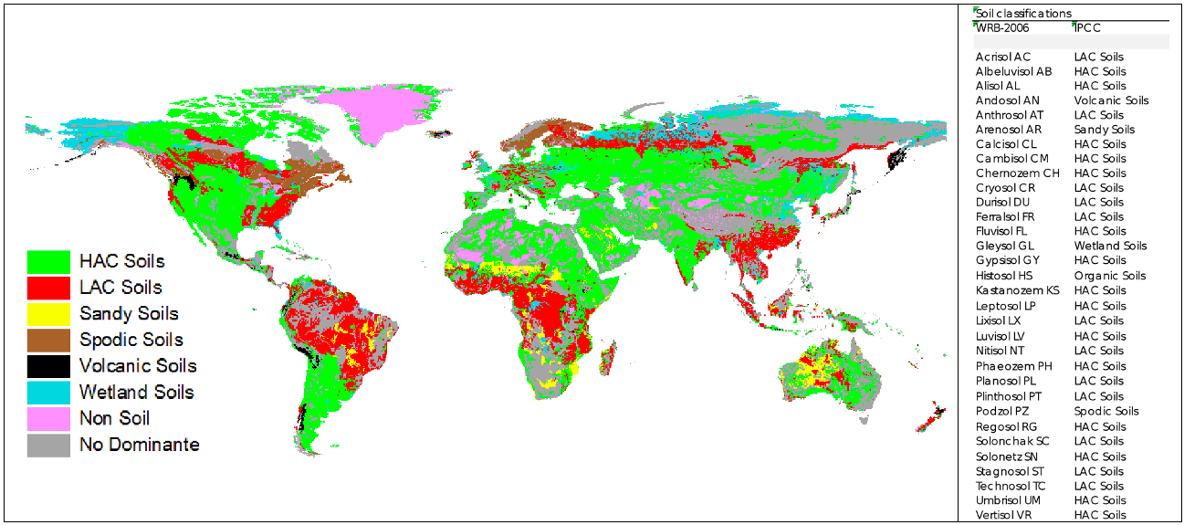
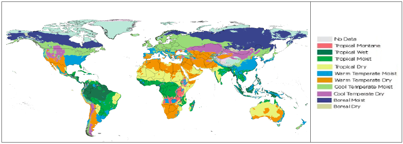
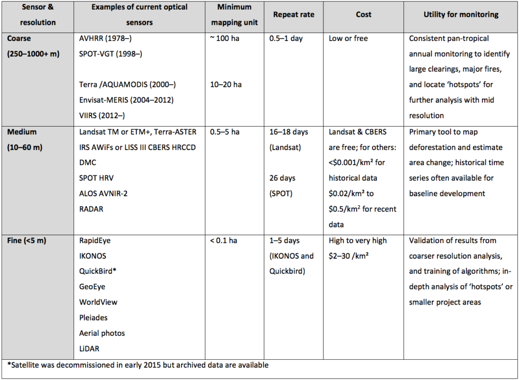
Remote sensing data
Approach 3 for representing land use areas generally requires remotely sensed data in combination with geo-referenced sampling based on field or household surveys. The table below summarizes existing remote-sensing data products (fig. 3).
Ground-based surveys
Management practices potentially affecting soil carbon stocks (such as tillage and input levels) generally cannot be ascertained from remote sensing data and may require land manager interviews or questionnaires.
Methods and sources of stock reference or stock change factors
- Hengl T, et al. 2017. SoilGrids250m: global gridded soil information based on Machine Learning. PLoS ONE.
- Hengl T, et al. 2014. SoilGrids1km — Global Soil Information Based on Automated Mapping. PLoS ONE.
- ICRAF’s Sentinel Landscapes project has high-resolution data on land cover and soil carbon for 10 landscapes across the globe.
- ISRIC’s SoilGrids project provides global predictions for organic carbon and bulk density at a resolution of 250m
- Ogle SM, et al. 2019. Climate and Soil Characteristics Determine Where No-Till Management Can Store Carbon in Soils and Mitigate Greenhouse Gas Emissions. Scientific Reports.
- Emission factors for specific agricultural practices. SAMPLES.
- Sanderman J, et al. 2017. The soil carbon debt of 12,000 years of human land use. PNAS.
- Country-specific estimates of soil carbon stocks and stock change factors generally require some component of measurement. Also, see the AgLED guidance on measuring.